Approximating a drag table
Goal of this article: build a usable .drg curve from what you actually have — a data sheet quoting
several BCs, or velocities measured downrange — and know how far to trust the result.
Nobody has measured your bullet, but you are not empty-handed. Tools → Approximate Drag Table offers two
routes, and the choice between them is decided by which data you hold:
| You have | Use |
|---|---|
| BCs quoted at several Mach numbers or velocities, as many data sheets publish | From BC Curve… |
| Velocities measured at several distances — radar, or chronographs downrange | From Measured Velocities… |
Both produce a .drg file that is used exactly like a measured one, and both are standalone dialogs:
they describe a projectile being characterised, which has nothing to do with any open shot, so they start
empty and follow the units of the last trajectory you created.
What both need first
The header fields are the same on both dialogs, and two of them are not optional:
| Field | Required | Why |
|---|---|---|
| Name | Yes | Written into the file; also the suggested file name |
| Weight | Yes | The curve is stored scaled by sectional density — weight is part of the scale |
| Diameter | Yes | The other half of the sectional density |
| Length | No | Carried into the file for spin drift and aerodynamic jump later |
| Source | No | A note about where the data came from. Defaults to BC curve on the BC dialog |
If a required field is missing you get a sentence saying which and why, not an exception — the validation is deliberately in front of the library call.
From a BC curve
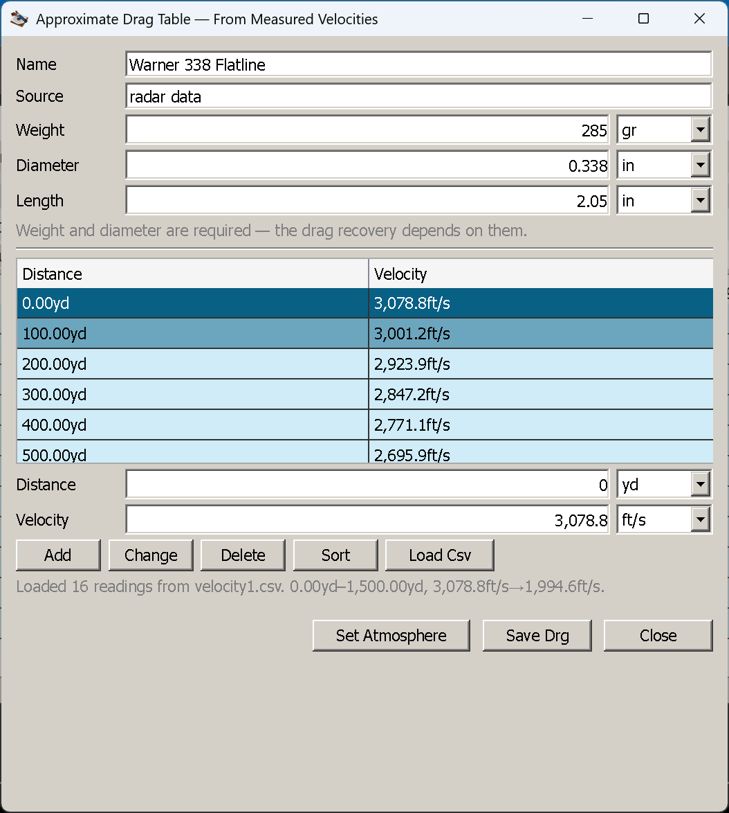
The velocities dialog with a real dataset loaded. The BC dialog has the same shape, with Mach and BC columns instead of distance and velocity.
The grid takes knots: a Mach number and the BC quoted at it. Add them with Add, correct one with Change, remove with Delete, and put them in order with Sort. Load Csv imports a two-column file.
Two details that matter:
- Knots are keyed by Mach, not velocity. A velocity would need an atmosphere to be meaningful; Mach is what the curve is actually a function of. The dialog shows a velocity column as a convenience — the conversion uses the atmosphere set with Set Atmosphere, standard air if you leave it alone.
- Each knot remembers the table its BC was quoted against, and the Base table dropdown (default
G7) says what the finished curve is scaled from. Knots quoted against a different standard table are converted at their own Mach when you save, and the confirmation tells you how many were. A knot quoted asGC, or as a form factor, cannot be converted and is refused with a reason.
So a data sheet giving G1 BCs at four velocities can be typed in as G1 knots and built against G7 without you converting anything by hand.
What you get: the standard base curve, reshaped so that it reproduces your BCs at the Mach numbers you gave. Between knots it interpolates; outside them it extends the base curve’s shape. Which means: the answer is only as good as the span your knots cover. Four knots from Mach 3 down to Mach 1.5 give a trustworthy curve over that band and a guess below it.
From measured velocities
The grid takes readings: a distance and the velocity measured there. Same buttons, plus the same Load Csv.
The requirements are stricter, because the maths is recovering drag from deceleration:
- At least three readings. Two points cannot describe a curve.
- Each distance must be distinct, and readings are sorted by distance.
- Velocity must decrease with distance. A rising velocity means transposed rows or a typo, and the dialog says so rather than producing nonsense. This catches the single most common data-entry error.
Set Atmosphere matters more here than on the BC dialog: the air the data was measured in drives the recovered coefficients, because drag depends on density. If your radar session was at 1,500 m on a hot day and you leave it at standard, every coefficient is wrong by that density ratio. Standard is assumed when you leave it alone — fine for a published dataset that says it was standardised, wrong for your own measurements.
What you get: a curve derived from your own bullet’s actual deceleration, which is the best thing on offer short of a manufacturer’s radar table. Its quality follows the data — more readings over a wider velocity span, measured in known air, give a better curve. Three readings 100 m apart describe one small piece of the curve and extrapolate the rest.
Saving
Save Drg validates, builds and writes the file, defaulting into data/drg with the name as the file
name. The confirmation reports how many points the table has, and how many knots were converted.
The file that comes out is a normal .drg: it carries the curve, the name, the source and the bullet
dimensions, and it records itself as a form factor of 1 on GC — the
convention that makes a measured curve the answer rather than a scaled
standard one. Attach it on the Ammunition tab with Browse… like any other.
How much to trust it
Say it plainly, because this is where a manual should not be encouraging:
- An approximated curve is better than a single BC over the range your data covers, and it is not better than a measured curve anywhere.
- It is at its worst exactly where you want it most: below the transonic region, where the standard curves diverge in shape and your knots or readings usually stop.
- It cannot invent information. Four knots is four facts and a lot of interpolation. If the resulting 1,000 yd drop differs from your observed drop, believe the target.
Use it as what it is: a better description of your bullet than a catalogue number, built from the data you happen to have, with the accuracy that implies.
Next
Converting a ballistic coefficient — the everyday G1 ↔ G7 question, and why a single converted number is always a compromise.